Putting several transmitters on one frequency on purpose means managing interference instead of avoiding it. This post touches on the science behind simulcast, and how coverage and timing are tuned in a real system.
Simulcast is controlled interference
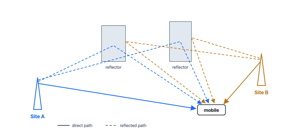
Every mobile radio already deals with interference from its own signal. At a single site, the signal reaches the radio by a direct path and also by reflections off buildings and terrain. The reflected copies arrive a little later and at a different strength. This is ordinary multipath, and receivers handle it every day.
Simulcast adds more of the same. A second site on the same frequency is, from the radio’s point of view, one more source of “reflections”: its direct path and its own reflections all land on top of the first site’s. This is co-channel multipath interference. The job of simulcast design is to keep that interference under control, so that where two sites overlap the radio still recovers clean audio or data.
What the receiver does with it
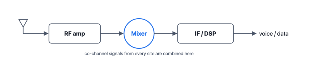
A receiver amplifies what arrives at its antenna, mixes it down to an intermediate frequency, and demodulates it. When two or more signals are on, or very nearly on, the same frequency, they go through the mixer together and come out combined. Distortion is added along the way. What the radio finally produces depends on how its demodulator handles that combined signal. Everything else in simulcast design exists to make sure that combination still demodulates cleanly.
Carrier frequency and phase
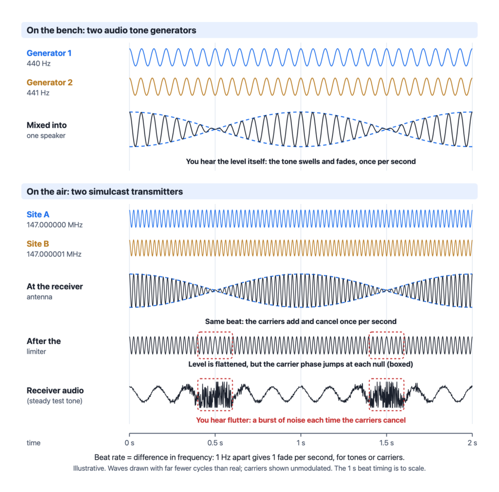
A mixer produces the sum and the difference of the signals fed into it. Put two transmitters at 147.000000 MHz and 147.000001 MHz, only 1 Hz apart, and the receiver sees a 1 Hz difference product. That is heard as a rolling fade, sometimes called “mobile flutter”.
Being frequency-locked is not the same as being phase-locked. To a receiver, a small change in phase looks just like a change in frequency, so a slow phase drift between sites also shows up as a rolling fade, and there is little that can be done about it at the receiver.
Hear this your self
You can reproduce the effect on a bench with two audio signal generators. Set one to 440 Hz and the other to 441 Hz at the same level, and mix them into a single speaker. The combined tone swells and fades once per second, because the two waves drift in and out of step, adding together and then cancelling. The beat rate is simply the difference between the two frequencies. Two carriers at 147.000000 and 147.000001 MHz beat at the same 1 Hz as the two tones.
This analogy has a limit. In the radio the beat happens to the RF carrier, before the audio is recovered. An FM receiver ignores changes in signal level, so the listener doesn’t hear a smooth swell. They hear the audio flutter and break into noise each time the two carriers cancel. Try turning one generator down: the fade becomes shallower. That is the capture effect at work, as described below. When one signal is much stronger than the other, the weaker one can barely pull it down.
Note: the demo needs both tones summed into one speaker or one channel, not one tone in each ear.
Audio timing: the 30-degree rule
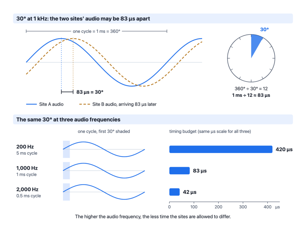
The decoded audio from each transmitter has to reach the radio within 30 degrees of phase of each other. Turning that into a time depends on the audio frequency. Using 1,000 Hz as the reference:
- 360° ÷ 30° = 12, so the budget is one twelfth of a cycle.
- A 1,000 Hz tone has a 1 ms period.
- 1 ms ÷ 12 ≈ 83 µs.
| Audio frequency | Period | 30° timing budget |
|---|---|---|
| 200 Hz | 5 ms | 420 µs |
| 1,000 Hz | 1 ms | 83 µs |
| 2,000 Hz | 0.5 ms | 42 µs |
The higher the audio frequency, the tighter the budget.
The same effect applies to data. For digital modulations, the limit is expressed as delay spread, and refers to the bit-error-rate versus delay-spread curves in TIA TSB-88. These show the error rate climbing as the delay spread between sites increases, with some modulations tolerating much more spread than others.
Capture effect and overlap
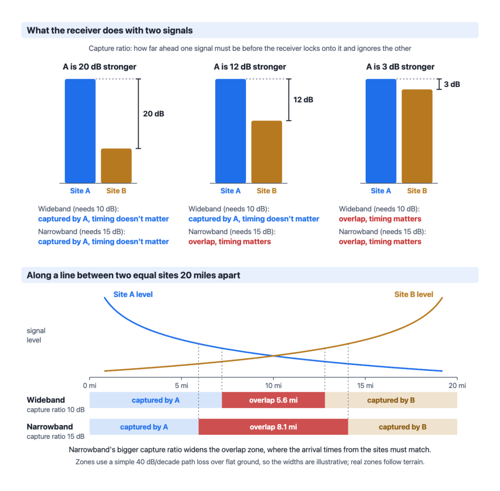
An FM detector will capture the stronger of two signals when their levels are different enough. It locks onto the stronger one and largely ignores the weaker. The narrower the deviation, the less capture effect there is.
This defines where timing matters. An overlap area is a place where no single transmitter is strong enough to capture the receiver. Only there does the delay between sites need to be managed. The thing that matters is the delay difference inside the overlap areas, not the distance between the transmitters.
The speed of radio adds up
Radio travels at about 5.4 µs per mile. That sounds quick, but the miles add up: 10 miles is 54 µs and 20 miles is 108 µs. Compare that with the 83 µs budget at 1 kHz. A path-length difference of 20 miles is already too much if the receiver is in an overlap area.
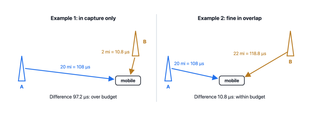
| Example | Path lengths | Arrival difference | Result |
|---|---|---|---|
| Two sites, mobile close to one | 20 mi / 2 mi | 97.2 µs | OK only if the near site captures the receiver |
| Two sites, mobile roughly equidistant | 20 mi / 22 mi | 10.8 µs | OK both in capture and in overlap |
| Three sites (C, A, B) | 40 / 10 / 5 mi | 189 µs (C–A), 27 µs (A–B) | A radio might be in overlap with all three. Avoid this by controlling coverage. |
The three-site case is closer to the real world. A pair of nearby sites can be well matched while a distant site’s signal arrives far too late. The is answer is to control where each site’s coverage goes, so a radio isn’t left in overlap with a far-off site.
Design it on the computer first
A coverage-prediction program for simulcast has to calculate time-delay interference as well as signal level. Design criteria:
| Modulation | Capture ratio | Maximum delay |
|---|---|---|
| Wideband analog FM | 10 dB | 80 µs |
| Narrowband analog FM | 15 dB | 80 µs |
| P25 C4FM (DAQ 3.4) | 15 dB | 30 µs |
| P25 LSM (DAQ 3.4) | 15 dB | 70 µs |
With those two numbers, a prediction can mark each place as either captured by one site (more than 15 dB stronger than the others, so delay doesn’t matter) or in overlap (where the arrival-time difference has to be within the delay limit). The 2016 talk also compared delay-interference predictions for the same system at wideband and narrowband deviation. Because narrower deviation gives less capture, deviation is one of the inputs that moves the overlap areas.
Antenna downtilt: a trade-off
Tilting a site’s antenna down clearly raises signal levels close to the site. It reduces the areas of overlap interference, but at a cost. High sites lose some of their wide-area coverage, so talk-out is reduced in some places. Simulcast from high sites is often difficult, and much of the reason for choosing a high site goes away once its coverage has to be pulled in.
You can’t tune a simulcast system by driving around. You need to model it in software.
Software modeling: delay spread
Salinas Valley Repeater Group uses its own in house modeling software to calculate and map the delay spread for our simulcast system. A delay spread map lets us visualize the differential delay or ‘delay spread’ within the designed coverage area of our system.
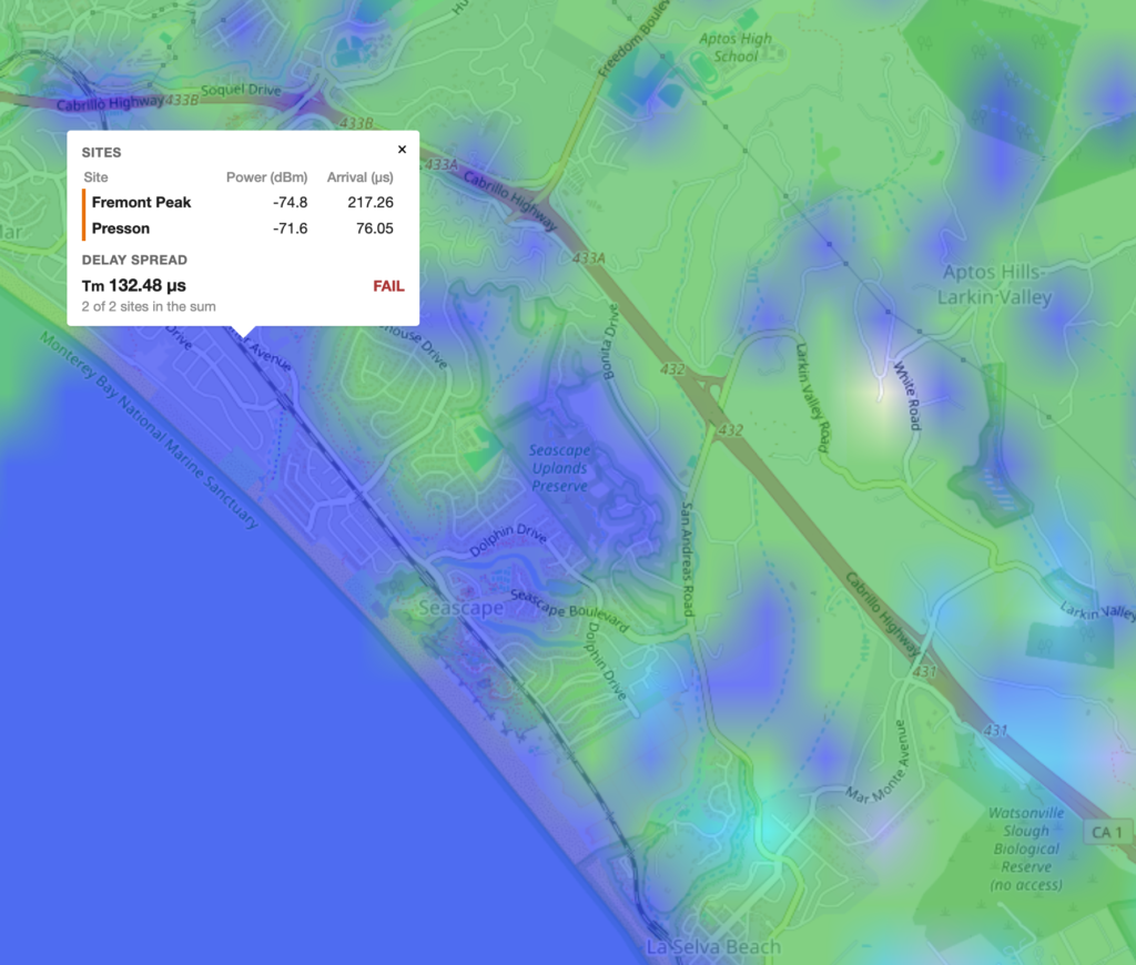
The map pictured shows an area in Santa Cruz County that will be out of our phase budget so the resulting signal in this area will have distortion artifacts.
reference sources
- Joe Blaschka Jr., PE, ADCOMM Engineering Company, “Simulcast – Theory or why we do the things we do,” Simulcast Forum XX, Las Vegas, 2016.
- Joe Blaschka Jr., PE, ADCOMM Engineering Company, “Simulcast – Propagation and Tuning,” Simulcast Forum XXII, Orlando, 2018.
- Both presentations are published by Simulcast Solutions in its Simulcast Forums / Case Studies collection: simulcastsolutions.com